代码
import stata_setup
stata_setup.config('C:/Program Files/Stata18', 'mp', splash=False)import stata_setup
stata_setup.config('C:/Program Files/Stata18', 'mp', splash=False)散点图是一种用于可视化两个变量之间关系的图形。它通过在二维坐标系中绘制点来表示数据点的位置,横轴和纵轴分别表示两个变量的值。散点图可以帮助我们识别变量之间的相关性、趋势和异常值。
散点图通常用于探索性数据分析(EDA)阶段。
%%stata
// 载入数据集,使用 Stata 的内置数据集 auto.dta
sysuse auto, clear
. // 载入数据集,使用 Stata 的内置数据集 auto.dta
. sysuse auto, clear
(1978 automobile data)

. Stata提供了多种 scheme (style)来美化图形。可以使用set scheme命令来设置主题。以下是一些常用的主题:
s1color:适用于需要强调数据点的情况,具有鲜艳的颜色。s2color:默认主题,适用于需要强调数据点的情况。s1mono:单色主题,适用于打印或黑白显示。s2mono:单色主题,适用于强调数据点的情况。economist:适用于经济学和社会科学领域的主题。journal:适用于学术期刊的主题,具有简洁和专业的外观。s1manual:手动主题,适用于需要自定义颜色和样式的情况。s2manual:手动主题,适用于强调数据点的情况。s2color8:适用于需要强调数据点的情况,具有8种颜色的主题。plotplain:适用于需要强调数据点的情况,具有简单和清晰的外观。更好的主题?
simono:适用于需要强调数据点的情况,具有简洁和专业的外观。
set scheme s1mono : 当前会话中设置主题为s1mono。
set scheme s1mono, perm : 永久设置主题为s1mono, perm 为 permanent 的缩写。
scatter命令用于绘制散点图。基本语法如下:
[twoway] scatter yvar xvar [if] [in] [weight] [, options]最基础的形式:
twoway scatter yvar xvar进阶形式:
twoway scatter y1 y2 y3 x1 x2 x3 [if] [in] [weight], options%%stata
twoway scatter mpg weight
%%stata
twoway scatter weight length price
twoway scatter y x,msymbol(oh) mcolor(red) msize(medium) scheme(s1mono)msymbol:改变形状(help symbolstyle)mcolor:改变颜色(help colorstyle)msize:改变大小(help markerstyle)%%stata
help symbolstyle
[G-4] symbolstyle -- Choices for the shape of markers
                     (View complete PDF manual entry)


Syntax
------

                        Synonym
        symbolstyle     (if any)     Description
        -------------------------------------------------------
        circle             O         solid
        diamond            D         solid
        triangle           T         solid
        square             S         solid
        plus               +
        X                  X
        arrowf             A         filled arrow head
        arrow              a
        pipe               |
        V                  V

        smcircle           o         solid
        smdiamond          d         solid
        smsquare           s         solid
        smtriangle         t         solid
        smplus
        smx                x
        smv                v

        circle_hollow      Oh        hollow
        diamond_hollow     Dh        hollow
        triangle_hollow    Th        hollow
        square_hollow      Sh        hollow

        smcircle_hollow    oh        hollow
        smdiamond_hollow   dh        hollow
        smtriangle_hollow  th        hollow
        smsquare_hollow    sh        hollow

        point              p         a small dot
        none               i         a symbol that is invisible
        -------------------------------------------------------

        For a symbol palette displaying each of the above symbols, type

            . palette symbolpalette [, scheme(schemename)]

        Other symbolstyles may be available; type

            . graph query symbolstyle

        to obtain the complete list of symbolstyles installed on your
        computer.


Description
-----------

    Markers are the ink used to mark where points are on a plot; see [G-3]
    marker_options.  symbolstyle specifies the shape of the marker.

    You specify the symbolstyle inside the msymbol() option allowed with many
    of the graph commands:

        . graph twoway ..., msymbol(symbolstyle) ...

    Sometimes you will see that a symbolstylelist is allowed:

        . scatter ..., msymbol(symbolstylelist) ...

    A symbolstylelist is a sequence of symbolstyles separated by spaces.
    Shorthands are allowed to make specifying the list easier; see [G-4]
    stylelists.


Links to PDF documentation
--------------------------

        Remarks and examples

    The above sections are not included in this help file.


Remarks
-------

    Remarks are presented under the following headings:

        Typical use
        Filled and hollow symbols
        Size of symbols


Typical use
-----------

    msymbol(symbolstyle) is one of the more commonly specified options.  For
    instance, you may not be satisfied with the default rendition of

        . scatter mpg weight if foreign ||
          scatter mpg weight if !foreign

    and prefer

        . scatter mpg weight if foreign, msymbol(oh) ||
          scatter mpg weight if !foreign, msymbol(x)

    When you are graphing multiple y variables in the same plot, you can
    specify a list of symbolstyles inside the msymbol() option:

        . scatter mpg1 mpg2 weight, msymbol(oh x)

    The result is the same as typing

        . scatter mpg1 weight, msymbol(oh) ||
          scatter mpg2 weight, msymbol(x)

    Also, in the above, we specified the symbol-style synonyms.  Whether you
    type

        . scatter mpg1 weight, msymbol(oh) ||
          scatter mpg2 weight, msymbol(x)

    or

        . scatter mpg1 weight, msymbol(smcircle_hollow) ||
          scatter mpg2 weight, msymbol(smx)

    makes no difference.


Filled and hollow symbols
-------------------------

    The symbolstyle specifies the shape of the symbol, and in that sense, one
    of the styles circle and hcircle -- and diamond and hdiamond, etc. -- is
    unnecessary in that each is a different rendition of the same shape.  The
    option mfcolor(colorstyle) (see [G-3] marker_options) specifies how the
    inside of the symbol is to be filled.  hcircle(), hdiamond, etc., are
    included for convenience and are equivalent to specifying

        msymbol(Oh): msymbol(O) mfcolor(none)

        msymbol(dh): msymbol(d) mfcolor(none)

        etc.

    Using mfcolor() to fill the inside of a symbol with different colors
    sometimes creates what are effectively new symbols.  For instance, if you
    take msymbol(O) and fill its interior with a lighter shade of the same
    color used to outline the shape, you obtain a pleasing result.  For
    instance, you might try

        msymbol(O) mlcolor(yellow) mfcolor(.5*yellow)

    or

        msymbol(O) mlcolor(gs5) mfcolor(gs12)

    as in

        . scatter mpg weight, msymbol(O) mlcolor(gs5) mfcolor(gs14)
          (click to run)


Size of symbols
---------------

    Just as msymbol(O) and msymbol(Oh) differ only in mfcolor(), msymbol(O)
    and msymbol(o) -- symbols circle and smcircle -- differ only in msize().
    In particular,

        msymbol(O): msymbol(O) msize(medium)

        msymbol(o): msymbol(O) msize(small)

    and the same is true for all the other large and small symbol pairs.

    msize() is interpreted as being relative to the size of the graph region
    (see [G-3] region_options), so the same symbol size will in fact be a
    little different in

        . scatter mpg weight

    and

. scatter mpg weight, by(foreign total)%%stata
help colorstyle
[G-4] colorstyle -- Choices for color
                    (View complete PDF manual entry)


Syntax
------

    Set color of <object> to colorstyle

        <object>color(colorstyle)


    Set color of all affected objects to colorstyle

        color(colorstyle)


    Set opacity of <object> to #, where # is a percentage of 100% opacity

        <object>color(%#)


    Set opacity for all affected objects colors to #

        color(%#)


    Set both color and opacity of <object>

        <object>color(colorstyle%#)


    Set both color and opacity of all affected objects

        <object>color(colorstyle%#)


    colorstyle            Description
    -------------------------------------------------------------------------
    black

    stc1                  color used by scheme stcolor
    stc2                  color used by scheme stcolor
    .
    .
    stc15                 color used by scheme stcolor
    stblue                blue used by scheme stcolor
    stgreen               green used by scheme stcolor
    stred                 red used by scheme stcolor
    styellow              yellow used by scheme stcolor

    gs0                   gray scale: 0 = black
    gs1                   gray scale: very dark gray
    gs2
    .
    .
    gs15                  gray scale: very light gray
    gs16                  gray scale: 16 = white

    white

    blue
    bluishgray
    brown
    cranberry
    cyan
    dimgray               between gs14 and gs15
    dkgreen               dark green
    dknavy                dark navy blue
    dkorange              dark orange
    eggshell
    emerald
    forest_green
    gold
    gray                  equivalent to gs8
    green
    khaki
    lavender
    lime
    ltblue                light blue
    ltbluishgray          light blue-gray, used by scheme s2color
    ltkhaki               light khaki
    magenta
    maroon
    midblue
    midgreen
    mint
    navy
    olive
    olive_teal
    orange
    orange_red
    pink
    purple
    red
    sand
    sandb                 bright sand
    sienna
    stone
    teal
    yellow

                          colors used by The Economist magazine:
    ebg                           background color
    ebblue                        bright blue
    edkblue                       dark blue
    eltblue                       light blue
    eltgreen                      light green
    emidblue                      midblue
    erose                         rose

    none                  no color; invisible; draws nothing
    background or bg      same color as background
    foreground or fg      same color as foreground

    "# # #"               RGB value; white = "255 255 255"

    "# # # #"             CMYK value; yellow = "0 0 255 0"

    "hsv # # #"           HSV value; white = "hsv 0 0 1"

    colorstyle*#          color with adjusted intensity; #'s range from 0 to
                            255

    colorstyle%#          color with adjusted opacity; #s range from 0 to 100

    *#                    default color with adjusted intensity
    %#                    default color with adjusted opacity
    -------------------------------------------------------------------------
    When specifying RGB, CMYK, or HSV values, it is best to enclose the
      values in quotes; type "128 128 128" not 128 128 128.


Description
-----------

    colorstyle sets the color and opacity of graph components such as lines,
    backgrounds, and bars.  Some options allow a sequence of colorstyles with
    colorstylelist; see [G-4] stylelists.


Links to PDF documentation
--------------------------

        Remarks and examples

    The above sections are not included in this help file.


Remarks
-------

    colorstyle sets the color and opacity of graph components such as lines,
    backgrounds, and bars.  Colors can be specified with a named color, such
    as black, olive, and yellow, or with a color value in the RGB, CMYK, or
    HSV format.  colorstyle can also set a component to match the background
    color or foreground color.  Additionally, colorstyle can modify color
    intensity, making the color lighter or darker.  Some options allow a
    sequence of colorstyles with colorstylelist; see [G-4] stylelists.

    To see a list of named colors, use graph query colorstyle.  See [G-2]
    graph query.  For a color palette showing an individual color or
    comparing two colors, use palette color.  See [G-2] palette.

    Remarks are presented under the following headings:

        Adjust opacity
        Adjust intensity
        Specify RGB values
        Specify CMYK values
        Specify HSV values
        Export custom colors


Adjust opacity
--------------

    Opacity is the percentage of a color that covers the background color.
    That is, 100% means that the color fully hides the background, and 0%
    means that the color has no coverage and is fully transparent.  If you
    prefer to think about transparency, opacity is the inverse of
    transparency.  Adjust opacity with the % modifier.  For example, type

        green%50
        "0 255 0%50"
        %30

    Omitting the color specification in the command adjusts the opacity of
    the object while retaining the default color.  For instance, specify
    mcolor(%30) with graph twoway scatter to use the default fill color at
    30% opacity.

    Specifying color%0 makes the object completely transparent and is
    equivalent to color none.


Adjust intensity
----------------

    Color intensity (brightness) can be modified by specifying a color, *,
    and a multiplier value.  For example, type

        green*.8
        purple*1.5
        "0 255 255*1.2"
        "hsv 240 1 1*.5"

    A value of 1 leaves the color unchanged, a value greater than 1 makes the
    color darker, and a value less than 1 makes the color lighter.  Note that
    there is no space between color and *, even when color is a numerical
    value for RGB or CMYK.

    Omitting the color specification in the command adjusts the intensity of
    the object's default color.  For instance, specify bcolor(*.7) with graph
    twoway bar to use the default fill color at reduced brightness, or
    specify bcolor(*2) to increase the brightness of the default color.

    Specifying color*0 makes the color as light as possible, but it is not
    equivalent to color none.  color*255 makes the color as dark as possible,
    although values much smaller than 255 usually achieve the same result.

    For an example using the intensity adjustment, see Typical use in [G-2]
    graph twoway kdensity.


RGB values
----------

    In addition to specifying named colors such as yellow, you can specify
    colors with RGB values.  An RGB value is a triplet of numbers ranging
    from 0 to 255 that describes the level of red, green, and blue light that
    must be emitted to produce a given color.  RGB is used to define colors
    for on-screen display and in nonprofessional printing.  Examples of RGB
    values are

        red     =   255    0    0
        green   =     0  255    0
        blue    =     0    0  255
        white   =   255  255  255
        black   =     0    0    0
        gray    =   128  128  128
        navy    =    26   71  111


CMYK values
-----------

    You can specify colors using CMYK values.  You will probably only use
    CMYK values when they are provided by a journal or publisher.  You can
    specify CMYK values either as integers from 0 to 255 or as proportions of
    ink using real numbers from 0.0 to 1.0.  If all four values are 1 or
    less, the numbers are taken to be proportions of ink.  For example,

        red     =     0  255  255    0   or, equivalently,     0     1  1     0
        green   =   255    0  255    0   or, equivalently,     1     0  1     0
        blue    =   255  255    0    0   or, equivalently,     1     1  0     0
        white   =     0    0    0    0   or, equivalently,     0     0  0     0
        black   =     0    0    0  255   or, equivalently,     0     0  0     1
        gray    =     0    0    0  128   or, equivalently,     0     0  0    .5
        navy    =    85   40    0  144   or, equivalently,  .334  .157  0  .565


HSV values
----------

    You can specify colors with HSV (hue, saturation, and value), also called
    HSL (hue, saturation, and luminance) and HSB (hue, saturation, and
    brightness).  HSV is often used in image editing software.  An HSV value
    is a triplet of numbers.  So that Stata can differentiate them from RGB
    values, HSV colors must be prefaced with hsv.  The first number specifies
    the hue from 0 to 360, the second number specifies the saturation from 0
    to 1, and the third number specifies the value (luminance or brightness)
    from 0 to 1.  For example,

        red     =   hsv   0     1     1
        green   =   hsv 120     1  .502
        blue    =   hsv 240     1     1
        white   =   hsv   0     0     1
        black   =   hsv   0     0     0
        navy    =   hsv 209  .766  .435


Export custom colors
--------------------

    graph export stores all colors as RGB+opacity values, that is, RGB values
    0-255 and opacity values 0-1.  If you need color values from Stata in
    CMYK format, use the graph export command with the cmyk(on) option, and
    save the graph in one of the following formats: PostScript, Encapsulated
    PostScript, or PDF.

    You can set Stata to permanently use CMYK colors for PostScript export
    files by typing translator set Graph2ps cmyk on and for EPS export files
    by typing translator set Graph2eps cmyk on.

    The CMYK values returned in graph export may differ from the CMYK values
    that you entered.  This is because Stata normalizes CMYK values by
    reducing all CMY values until one value is 0.  The difference is added to
    the K (black) value.  For example, Stata normalizes the CMYK value 10 10
    5 0 to 5 5 0 5.  Stata subtracts 5 from the CMY values so that Y is 0 and
    then adds 5 to K.


Video example
-------------

Transparency in Stata graphs%%stata
twoway scatter mpg weight,msymbol(D) mcolor(red) msize(medium)
按照某个变量分组绘制散点图,可以使用by选项。by选项可以将数据按照指定变量进行分组,并为每个组绘制单独的散点图。
twoway scatter y x, by(groupvar)%%stata
twoway scatter mpg weight,by(foreign)
%%stata
twoway(scatter mpg weight if foreign ==0)(scatter mpg weight if foreign ==1),legend(label(1 "Domestic") label(2 "Foreign"))
平滑曲线可以用来描述数据的变化趋势或者揭示数据中的隐藏模式。
在Stata中,绘制光滑曲线的命令主要有以下几种:lowess、loess、lowess2、lpoly和bspline。它们各自具有不同的特点和适用范围,可以根据具体的数据类型和分析目的选择使用。
lowess是一种局部加权回归平滑方法,它可以通过对数据集进行局部加权回归来生成光滑曲线。
lowess yvar xvar [if] [in] [, options]其中,yvar 是因变量,xvar 是自变量。options 是一些可选参数,用来进一步调整光滑曲线的形状和拟合效果。例如,可以通过指定 span 参数来控制局部回归的窗口大小,较小的 span 值会导致更平滑的曲线,而较大的 span 值会导致更接近原始数据的曲线。
options 有如下选项:
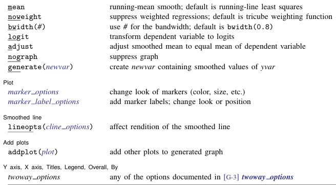
lowess 命令生成的光滑曲线可以通过绘图命令来展示,例如使用 twoway scatter 命令可以在散点图上叠加绘制光滑曲线。lowess — Lowess smoothing
lowess 命令的示例:%%stata
sysuse auto
lowess mpg weight, gen(lowess_mpg)
twoway scatter mpg weight || line lowess_mpg weight
. sysuse auto
(1978 automobile data)

. lowess mpg weight, gen(lowess_mpg)

. twoway scatter mpg weight || line lowess_mpg weight

. 
上述代码首先载入Stata自带的汽车数据集auto,然后使用lowess命令生成一个光滑曲线,将结果保存在变量lowess_mpg中。最后利用twoway scatter命令绘制散点图,并使用line命令在散点图上叠加绘制光滑曲线。