参数检验

作者

Simonzhou

发布于

2025年2月24日

1 参数检验

1.1 参数检验和非参数检验的区别

维度	参数检验（Parameter test）	非参数检验（Non-parameter tests）
定义	以特定的总体分布为前提$\rightarrow$?	不依赖于总体分布特征$\rightarrow$?
举例	$Z$检验、$t$分布、$F$检验	秩和检验（Rank sum test）、卡方检验
优点	1. 直接利用原始观测值计算统计量，检验效能高； 2.可对总体参数做出估计	1. 适用范围广、收集资料方便； 2. 多数非参数检验方法比较简便、易于掌握
缺点	对数据分布有特定要求，适用范围窄	1. 没有充分利用原始数据，检验效能低； 2. 不能对总体参数做出推断
适用范围	必须符合相应的要求，如两样本t检验要求：独立、正态、方差齐	1. 总体分布形式未知、分布类型不明确、偏态分布数据； 2. 等级资料； 3. 不满足参数检验条件的数据； 4. 数据一段或两端为无法测量的数值等。
选用原则	1. 如果数据符合参数检验条件，或经过变换后符合参数检验的条件，最好用参数检验； 2. 参数检验误用为非参数检验，会导致检验效能降低。

1.2 $t$分布

类目	$t$分布
概念	设从正态分布$N(\mu,\sigma^2)$随机抽取含量为n的样本，样本均数为$\bar x$、标准差为$s$、则$t=\frac{\bar x-\mu}{s_{\bar x}}=\frac{\bar x-\mu}{s/\sqrt{n}}$，自由度为$n-1$。
图形特点	一簇以0为中心，左右对称的单峰曲线；但随着自由度的增加，$t$分布曲线将越来越接近于标准正态分布曲线
统计量值	$t$的取值范围$-\infty \sim +\infty$
自由度	$v=n-1$

t-Distribution Curves vs. Standard Normal Curve

1.3 一个正态总体参数的估计

1.3.1 点估计

1.3.2 区间估计

总体均数$\mu$的置信区间估计

正态（或正态近似法）
t分布法

总体方差$\sigma^2$的置信区间估计

1.4 两个正态总体的参数估计

1.5 小结

样本均数的中心极限定理。从任意均数等于$\mu$，方差等于$\sigma^2$的一个总体中抽取样本量为$n$的简单随机样本，当样本量$n$很大时，无论总体分布形态如何，样本均数的抽样分布近似服从正态分布。
样本率的中心极限定理。从“成功”率为$\pi$的总体中随机抽取样本量为$n$的样本，其样本“成功”率用$p$表示，当$n\pi>5$且$n(1-\pi)>5$时，样本率$p$近似服从正态分布。

--- title: "参数检验" author: "Simonzhou" date: "2025-02-24" #format: # html: # 输出格式为 HTML # self-contained: true # 生成独立的 HTML 文件 # pdf: # 可选：如果需要 PDF 输出 # default execute: echo: true # 在输出中显示代码 eval: true # 执行代码 warning: false # 隐藏警告信息 message: false # 隐藏消息 cache: true # 启用代码缓存 freeze: true # 冻结代码输出 --- # 参数检验 ## 参数检验和非参数检验的区别 | 维度 | 参数检验（Parameter test） | 非参数检验（Non-parameter tests） | |:-----------------|:--------------------------|:--------------------------| | 定义 | 以特定的总体分布为前提$\rightarrow$? | 不依赖于总体分布特征$\rightarrow$? | | 举例 | $Z$检验、$t$分布、$F$检验 | 秩和检验（Rank sum test）、卡方检验 | | 优点 | 1\. 直接利用原始观测值计算统计量，检验效能高； 2.可对总体参数做出估计 | 1\. 适用范围广、收集资料方便； 2. 多数非参数检验方法比较简便、易于掌握 | | 缺点 | 对数据分布有特定要求，适用范围窄 | 1\. 没有充分利用原始数据，检验效能低； 2. 不能对总体参数做出推断 | | 适用范围 | 必须符合相应的要求，如两样本t检验要求：独立、正态、方差齐 | 1\. 总体分布形式未知、分布类型不明确、偏态分布数据； 2. 等级资料； 3. 不满足参数检验条件的数据； 4. 数据一段或两端为无法测量的数值等。 | | 选用原则 | 1\. 如果数据符合参数检验条件，或经过变换后符合参数检验的条件，最好用参数检验； 2. 参数检验误用为非参数检验，会导致检验效能降低。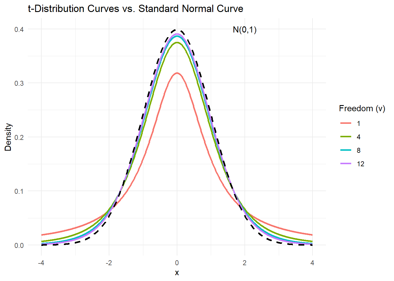 | | ## $t$分布 | 类目 | $t$分布 | |:--------------------------|:--------------------------------------------| | 概念 | 设从正态分布$N(\mu,\sigma^2)$随机抽取含量为n的样本，样本均数为$\bar x$、标准差为$s$、则$t=\frac{\bar x-\mu}{s_{\bar x}}=\frac{\bar x-\mu}{s/\sqrt{n}}$，自由度为$n-1$。 | | 图形特点 | 一簇以0为中心，左右对称的单峰曲线； 但随着自由度的增加，$t$分布曲线将越来越接近于标准正态分布曲线 | | 统计量值 | $t$的取值范围$-\infty \sim +\infty$ | | 自由度 | $v=n-1$ | ```{r ,fig.cap="t-Distribution Curves vs. Standard Normal Curve",fig.show='hold', fig.align='center', echo=FALSE} library(ggplot2) # Generate x-axis values x <- seq(-4, 4, length.out = 1000) # Degrees of freedom df_values <- c(1, 4, 8, 12) # Create a data frame for the t-distribution curves t_dist_data <- data.frame(x = rep(x, each = length(df_values)), df = rep(df_values, times = length(x))) # Calculate t-distribution probability density values t_dist_data$density <- dt(t_dist_data$x, df = t_dist_data$df) # Create a data frame for the standard normal distribution curve normal_data <- data.frame(x = x) normal_data$density <- dnorm(normal_data$x) # Create a ggplot for t-distribution curves with different colors t_dist_plot <- ggplot() + geom_line(data = t_dist_data, aes(x = x, y = density, color = factor(df)), size = 1) + geom_line(data = normal_data, aes(x = x, y = density), color = "black", size = 1, linetype = "dashed") + labs(title = "t-Distribution Curves vs. Standard Normal Curve", x = "x", y = "Density") + scale_color_discrete(name = "Freedom (v)", labels = c("1", "4", "8", "12", "Standard Normal")) + theme_minimal() + annotate("text", x = 2, y = 0.4, label = "N(0,1)", color = "black") # Display the t-distribution plot print(t_dist_plot) ``` ## 一个正态总体参数的估计 ### 点估计 ### 区间估计 #### 总体均数$\mu$的置信区间估计 1. 正态（或正态近似法） 2. t分布法 #### 总体方差$\sigma^2$的置信区间估计 ## 两个正态总体的参数估计 ## 小结 1. 样本均数的中心极限定理。从任意均数等于$\mu$，方差等于$\sigma^2$的一个总体中抽取样本量为$n$的简单随机样本，当样本量$n$很大时，无论总体分布形态如何，样本均数的抽样分布近似服从正态分布。 2. 样本率的中心极限定理。从“成功”率为$\pi$的总体中随机抽取样本量为$n$的样本，其样本“成功”率用$p$表示，当$n\pi>5$且$n(1-\pi)>5$时，样本率$p$近似服从正态分布。 end.